Level 3 AI in trading · Part 8/8

Feature Importance and Bet Sizing

Two closing questions that go beyond model quality: why does a model work, and how does its output become a position?

Why feature importance matters more than accuracy

At the signal-to-noise ratio of financial markets, the accuracy of a model only says so much. Two models with identical hit rates can rest on completely different features – one on a quantity that makes economic sense, the other on an artifact of data preparation.

Analyzing feature importance is therefore not a step you do at the end. It is the actual research output, and the only place where a model explains something.

Three methods

Mean decrease impurity (MDI). For tree methods: how much did a feature improve the splits across all trees? Fast, but with two known biases. Features with many possible values are favored, and the values refer to training data only.

Mean decrease accuracy (MDA). The values of one feature are shuffled after training, and you measure how much test performance drops. It refers to unseen data and works with any model. It has to run on purged splits, otherwise you measure the leakage along with it.

Single feature importance. Each feature is evaluated on its own as the only predictor. This avoids the substitution effect completely, but it misses features that only work in combination.

The substitution effect

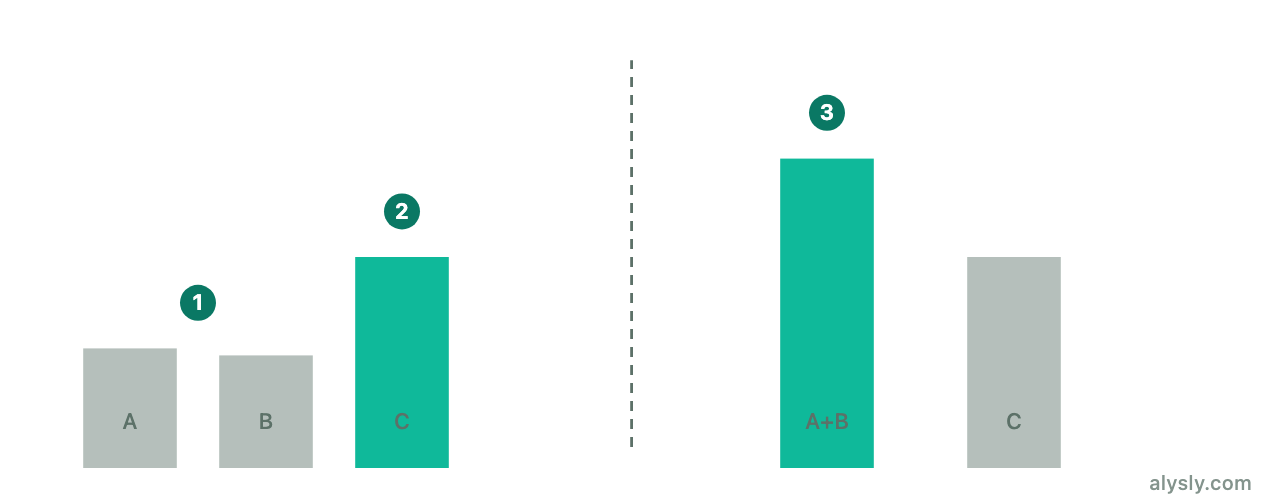
This is the most important trap in interpretation. When two features are strongly correlated – a 20-period and a 25-period average, for instance – they share the importance between them. Both look mediocre, even though the underlying information is central. The other way around, a single uncorrelated feature can look large without being especially valuable.

Importance of three features when two of them measure the same thing, and after grouping — On the left are three features, two of which measure nearly the same thing — say a 20-day and a 22-day average. (1) Both receive only a small importance score, because the forest picks one or the other and the effect splits between them. (2) Feature C therefore looks like the most important one, which it is not. (3) Group the two twins together and score the group as a whole, and the picture reverses. That is the substitution effect: a ranking of individual features measures not just usefulness but also how many relatives a feature has.

Level 2 already describes the same trap informally: five indicators from the same price series are not five independent opinions.

The usual way to handle it is to cluster correlated features first and measure the importance per cluster. The answer is then no longer “feature 17 matters” but “the cluster of trend measures matters” – a statement that still holds tomorrow. How strongly market quantities move together can be read directly from the correlation matrix .

From probability to position

A classification model outputs a probability, not a quantity. The step that translates one into the other helps determine the result.

Two principles:

Size in proportion to confidence. Instead of trading every position at the same size, you derive the size from the model probability: close to zero around 50 percent, growing as confidence rises. The common implementation maps the distance from 50 percent through a normal distribution function onto a value between 0 and 1.

The ceiling comes from risk, not from probability. The confidence of the model sets the share of the maximum position. The maximum itself comes from the risk calculation in Level 1 . A very confident signal does not justify a position that damages the account when it fails.

There is also a practical question that tends to disappear in backtests. When several signals run at the same time, their sizes have to be aggregated. Otherwise many small, correlated positions add up to one large risk.

Closing the course

Three levels, one continuous thread. Level 1 describes what a chart shows. Level 2 makes the patterns precise enough to be testable. Level 3 shows what that testing looks like when you take it seriously – and how many ways there are to fool yourself along the way.

The sober summary: most of the work in this field is not about finding edges but about ruling out apparent ones. Skip that part and you will always find something, and you will not keep it.

Tools on this site

Backtester — portfolio ideas against historical data
Monte Carlo tool — a range instead of a single path
Correlation matrix — how closely markets move together
Return triangle — the outcome as a function of entry and exit timing

Sources

The methods in this level come from the literature on financial machine learning, in particular Marcos López de Prado: Advances in Financial Machine Learning (Wiley 2018) and the accompanying ORIE 5256 lecture series, The 7 Reasons Most Machine Learning Funds Fail, and The Probability of Backtest Overfitting (Bailey, Borwein, López de Prado, Zhu). The presentation, examples and graphics here are our own.