Monte Carlo Savings Simulator
A standard savings calculator grows the balance by the same rate every year. Markets do not behave that way. This simulation runs the same savings plan 2,000 times with randomly fluctuating monthly returns and shows how far apart the outcomes can end up.
How the Simulation Works
The inputs are starting capital, monthly contribution, time horizon, expected return, volatility and a target amount. For every month, the simulation draws a return from a normal distribution. Its mean is the annual return divided by 12, and its spread is the annual volatility divided by the square root of 12. The balance grows by that return, and then the contribution is added. If the balance would drop below zero, it stays at zero.
After 2,000 paths, the simulation sorts the final values and reads off three points:
- Pessimistic (10%): 10% of the paths ended lower, 90% higher.
- Median (50%): half ended below this value, half above.
- Optimistic (90%): only 10% of the paths ended higher.
The chance of reaching the target is the share of paths that ended at or above the target amount. The chart shows these three points for every year as a fan.
Worked Example
€10,000 starting capital, €300 a month, 20 years, a 7% expected return and a €200,000 target. The amount paid in is €82,000. Every run draws new random numbers, so the figures shift by a few thousand euros from one run to the next.
| Volatility | 10% | Median | 90% | Chance of €200,000 |
|---|---|---|---|---|
| 5% | about €158,000 | about €194,000 | about €239,000 | about 42% |
| 15% | about €97,000 | about €173,000 | about €326,000 | about 38% |
| 25% | about €57,000 | about €139,000 | about €395,000 | about 32% |
A steady 7% return would produce about €197,000. The median lands below that, and further below the more returns swing. The reason is arithmetic: after a 20% loss, it takes a 25% gain to get back to the starting point. Volatility costs growth even when the average return stays the same. For context from our price series: the S&P 500 fluctuated by about 16% a year from 2017 to 2026, measured on monthly returns. Bitcoin came to about 45% since July 2024.
Limits of the Model
- Normal distribution. Real monthly returns have extreme outliers more often than a normal distribution assumes. Crashes like 2008 or March 2020 are rarer in the model than in reality.
- Independent months. Every month is a fresh draw. Long downturns with several bad months in a row only appear by chance.
- No costs or taxes. The expected return should already be net of costs. Taxes are not deducted.
- The inputs decide everything. Return and volatility are assumptions. The simulation shows how widely results spread under those assumptions, not what return a market will deliver.
The ETF savings plan calculator shows the steady calculation without fluctuations. The return triangle shows how actual annual returns were spread across past buy and sell years.
More calculators and tools are listed in the tools overview.
Latest Investment Analysis
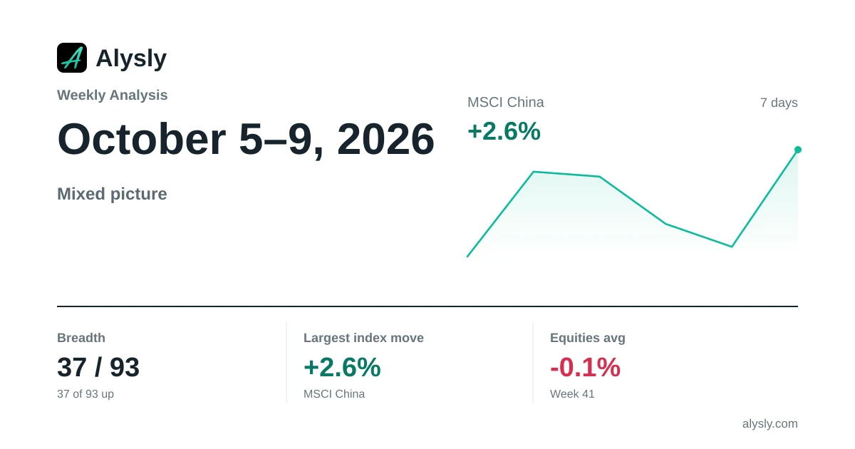 · Mixed
Weekly Analysis: MSCI China Leads the Week (+2.6%) · October 5–9, 2026
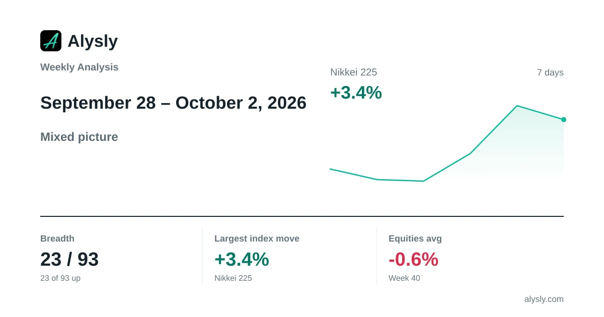 · Mixed
Weekly Analysis: Nikkei 225 Sets the Tone for the Week (+3.4%) · September 28 – October 2, 2026
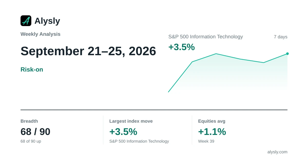 · Risk-on
Weekly Analysis: S&P 500 Information Technology Leads the Week (+3.5%) · September 21–25, 2026
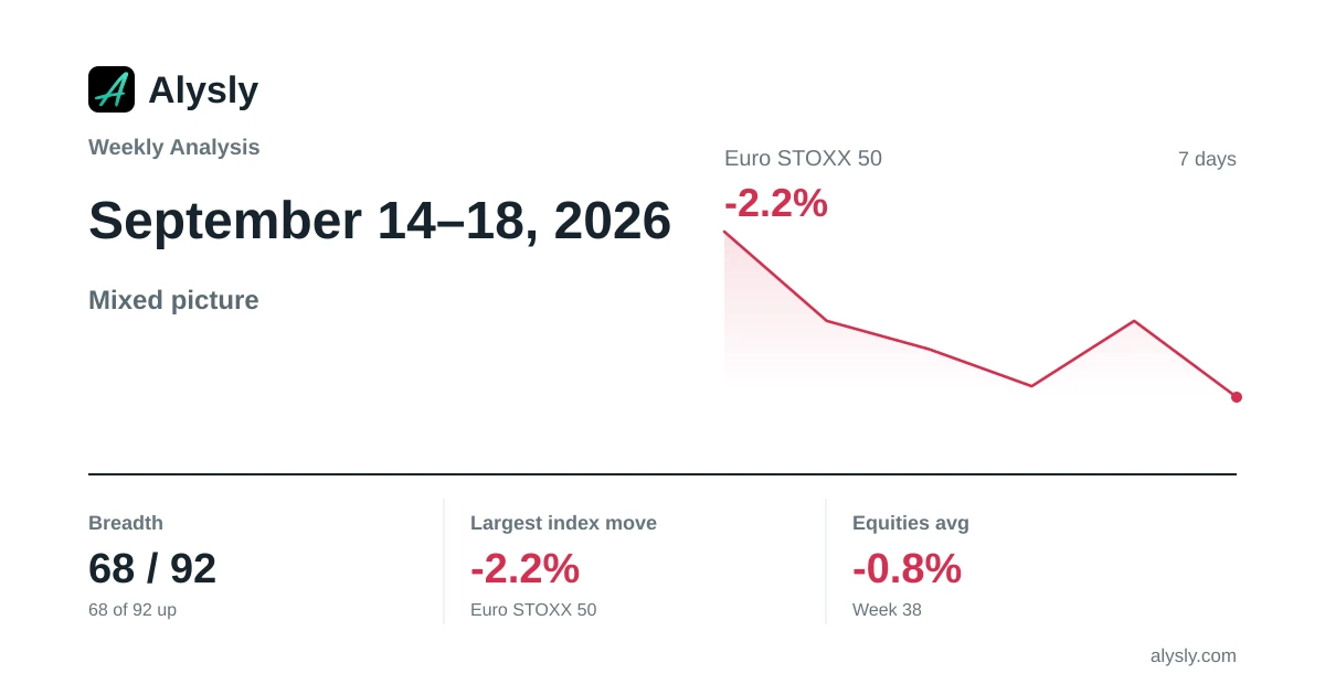 · Mixed
Weekly Analysis: Euro STOXX 50 Weighs on the Week (-2.2%) · September 14–18, 2026
 · Risk-off
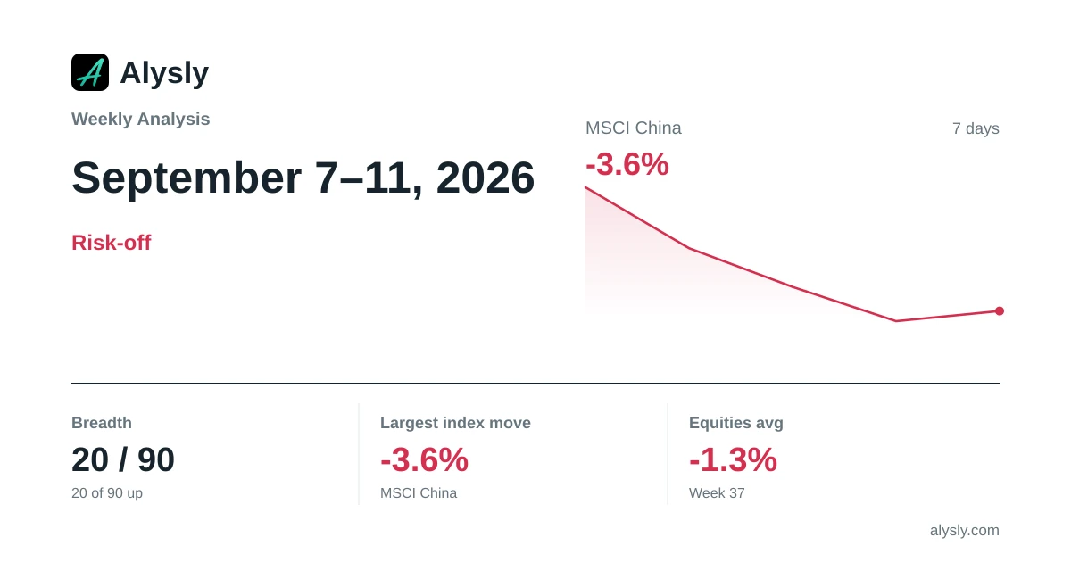
Weekly Analysis: MSCI China Lags the Week (-3.6%) · September 7–11, 2026