Level 2 Patterns & indicators · Part 9/9

Testing a Pattern

Up to this point the course has been descriptive. This article is the transition: it turns an observation into a statement that can be wrong.

Step 1: make the rule unambiguous

A pattern is only testable when a program can find it without judgment. “A hammer after a downtrend” is not enough. A testable version would be:

Lower wick at least twice the body, upper wick at most a quarter of the body, and the close below the 20-period average.

Every number in that definition is a decision. Those decisions become the problem later – but without them there is nothing to measure.

Step 2: define the outcome

What exactly are you measuring? “The price rises afterwards” is not a definition. You need three things: a horizon, a threshold and a comparison. For example: is the close 10 periods later at least 1 ATR higher?

A worse version is surprisingly common: the price is only checked after a fixed horizon. A path that falls far below any sensible stop in between and recovers at the end still counts as a success, even though in practice you would have been stopped out. Level 3 shows how to do this better with the triple-barrier method .

Step 3: establish the base rate

This is the most important step and the one most often skipped. Before you measure how often the pattern works, you have to know how often the same outcome happens without it.

If the price rises in 54 percent of all ten-period windows, then a pattern with a hit rate of 56 percent is not a discovery but noise. The hit rates published in pattern books almost never state a base rate – and without one, a percentage means nothing.

Four ways to fool yourself

Look-ahead bias. The calculation uses information that was not available at the time of the decision. The classic case: the close of the signal candle goes into the entry, although it is only known at the end of the period. The error is small, but it behaves like an edge.

Survivorship bias. The sample only contains instruments that still exist today. Bankruptcies and delistings are missing – and with them exactly the cases where everything went wrong.

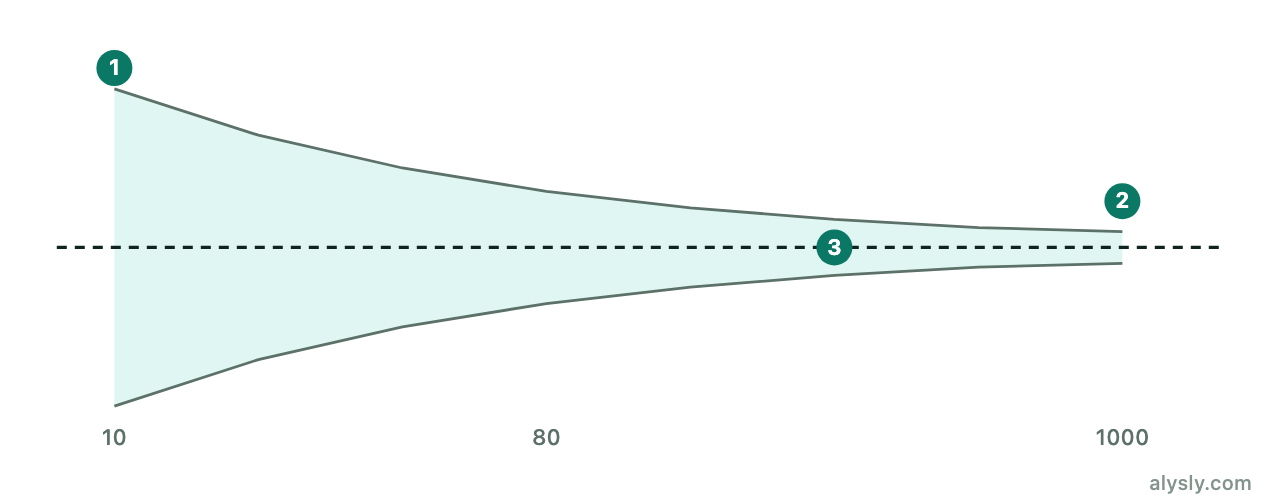
A sample that is too small. Thirty occurrences support no statement about a hit rate. With 30 observations, the confidence interval around a measured 60 percent runs roughly from 41 to 77 percent – a range that covers everything from useless to excellent.

Multiple testing. You try twenty variants, find a good one and report that one. This is the most expensive mistake in the whole discipline, and it is the reason Level 3 is almost entirely about it.

Step 4: separate development and testing

You develop the rule on one period and test it on another that you did not look at during development. That sounds obvious, and it is rarely done cleanly. The usual reason is that the test period gets used “one more time” after a disappointing first result. From the second look onwards it is no longer a test period.

For price data, the simple random split that is common in machine learning is not enough: price series depend on time, and neighboring observations overlap. Why the whole procedure fails on that, and how financial research repairs it, is the subject of Level 3 .

What a backtest can and cannot show

It can show that a rule did not work in the past. That is a solid result, and the most common one.

It cannot show that a rule will work in the future. At best it shows that the rule worked during one particular period – and how much that result is worth depends almost entirely on how many variants you tried before you found this one.

To put a portfolio idea against historical data right away, use the backtester and the Monte Carlo tool . The second one shows the range of outcomes the same statistics could just as easily have produced, instead of a single path.

Next

That is the end of Level 2. Level 3 picks up exactly this thread: what happens when you hand the testing to a machine, and why standard machine learning fails on financial data.