Level 3 AI in trading · Part 5/9
Labels: Triple Barrier and Meta-Labeling
The question a model is supposed to answer is usually settled in two lines of code and then never looked at again. It is the decision with the biggest consequences in the whole pipeline.
Why the fixed horizon fails
The standard approach asks: “is the price higher in ten periods?” It has one flaw that invalidates every later evaluation – it ignores the path.
Two paths with identical labels:
- Path A rises steadily by 3 percent.
- Path B falls 12 percent in between and ends 3 percent higher.
For the model, both are wins. In practice B is a loss, because any sensible risk management would have stopped out long before. A model trained on such labels learns to prefer situations that you could not actually hold.
The triple-barrier method
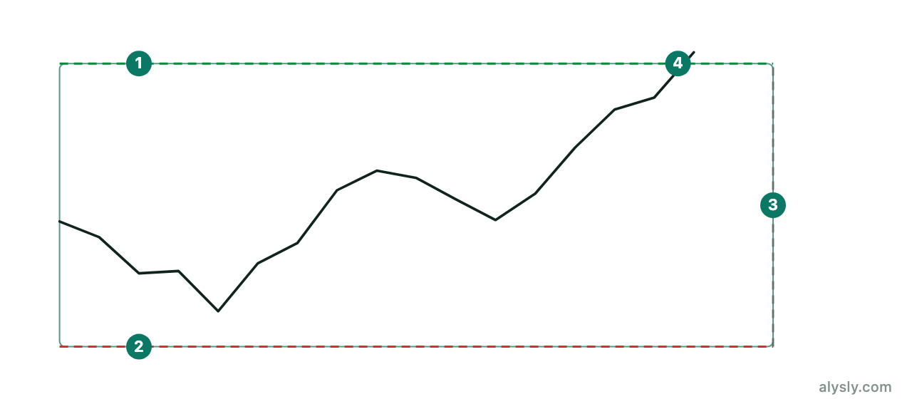
Instead of asking after a fixed horizon, you set three limits and ask which one is touched first:
- an upper limit (profit target),
- a lower limit (loss limit),
- a vertical limit (maximum holding time).
The label follows from whichever limit comes first: +1, −1 or 0. It therefore reproduces exactly what would have happened to a real position.
One addition matters: the barriers are set relative to volatility, for example as a multiple of the current ATR . With fixed percentage barriers you get almost nothing but time-limit labels in quiet phases and almost nothing but hits in volatile ones. The model then mainly learns the volatility regime.
Meta-labeling
A second idea splits the problem in a different way.
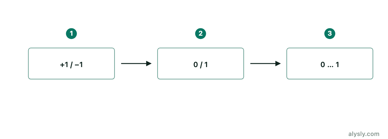
A primary model – or a simple rule, such as a crossover from Level 2 – decides the direction only. A secondary model then answers one binary question: is this signal likely to be correct? Its probability becomes the position size, anywhere between zero and full.
The benefit lies in the division of labor:
- The direction question is hard and full of noise. It stays with a rule you understand.
- The question “how reliable is this signal?” is far easier to learn, because it is asked in a context the secondary model can fill with features: volatility, regime, time of day, trend strength.
- The secondary model is allowed to set the size to zero. It can prevent damage without ever second-guessing the direction.
In practice, meta-labeling usually does not improve the hit rate but the ratio of win to loss, because it filters out the weak signals. In the language of Level 1 : it raises the expectancy per trade, not the number of winners.
The side effect
Both methods create a problem that the next article covers. When a label runs until a barrier is touched, neighboring examples overlap. Two observations one period apart share almost their entire outcome window, so they are anything but independent.
Next
Exactly that overlap, and how sample weights handle it.