Level 3 AI in trading · Part 5/8

Overlapping Examples and Sample Weights

Almost every standard machine learning method assumes that training examples are drawn independently. On financial data that assumption is nowhere near met, and the problem is not small but dominant.

Where the dependence comes from

If a label covers the next ten periods, two neighboring examples share nine of those ten. Their outcomes are driven by largely the same price moves.

To a model that looks like confirmation: the same relationship, again and again. In reality it is one observation entered ten times. The effective sample size is therefore far smaller than the number of rows, and any confidence statement based on the row count is correspondingly too narrow.

Uniqueness

The fix starts with a measurement. For each point in time, count how many labels cover it at the same time. An example whose outcome window overlaps many others is barely unique; one that stands alone is fully unique.

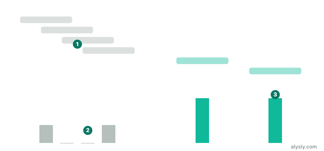
Overlapping label windows on a timeline and the observation weights that follow from them — Each bar at the top is the window over which one label is formed — ten days here. (1) The front windows overlap heavily: they describe largely the same price moves. To a model they still look like independent observations — that is the assumption breaking. (2) Below each observation is its uniqueness: the share of its window no other window touches. For the two middle ones it is zero — they are fully covered by their neighbours and add nothing of their own. (3) Free-standing windows get the full weight. These values serve as sample weights so that tightly packed observations do not count like many independent ones.

The average uniqueness across its window gives every example a weight. During training, examples with heavy overlap then count for less. The effect is unspectacular and important: the model stops mistaking repetition for evidence.

Weighting by the size of the outcome

A second, independent weighting: examples whose move was large carry more information than examples that barely cleared the noise. A common choice is to weight by the absolute return over the outcome window, divided by the number of labels running at the same time.

Taken together, uniqueness and size bring the training closer to what matters economically.

Time decay

Markets change. A relationship from 2011 is not wrong, but it is probably less relevant than one from last year. A time weight that decays linearly or exponentially accounts for that.

The setting is a trade-off, not an optimization problem. Strong decay makes the model adaptive and unstable; weak decay makes it stable and slow. What matters is only that you make the decision deliberately and do not tune it on the test data, because that would be the next way to burn through it.

Sequential bootstrap

Bagging methods such as random forests draw training examples at random with replacement. With overlapping data, almost identical examples land in the same draw, and the trees of a forest become more similar than intended. The whole advantage of the ensemble shrinks.

The sequential bootstrap corrects this: the probability of drawing an example falls once an overlapping example has already been drawn. The result is draws with considerably higher average uniqueness, and ensembles whose members really do differ.

The practical core

All three corrections do the same thing: they stop repetition from being counted as confirmation. That is the same error Level 2 describes for small samples – here written down formally and made measurable.

The same overlap also ruins validation. How to repair it is the next article.